How to Use a Oscilloscope
Introduction
Have you ever found yourself troubleshooting a circuit, needing more information than a simple multimeter can provide? If you need to uncover information like frequency, noise, amplitude, or any other characteristic that might change over time, you need an oscilloscope!
O-scopes are an important tool in any electrical engineer’s lab. They allow you to see electric signals as they vary over time, which can be critical in diagnosing why your 555 timer circuit isn’t blinking correctly, or why your noise maker isn’t reaching maximum annoyance levels.
Covered in This Tutorial
This tutorial aims to introduce the concepts, terminology, and control systems of oscilloscopes. It’s broken down into the following sections:
- Basics of O-Scopes – An introduction to what, exactly, oscilloscopes are, what they measure, and why we use them.
- Oscilloscope Lexicon – A glossary covering some of the more common oscilloscope characteristics.
- Anatomy of an O-Scope – An overview of the most critical systems on an oscilloscope – the screen, horizontal and vertical controls, triggers, and probes.
- Using an Oscilloscope – Tips and tricks for someone using an oscilloscope for the first time.
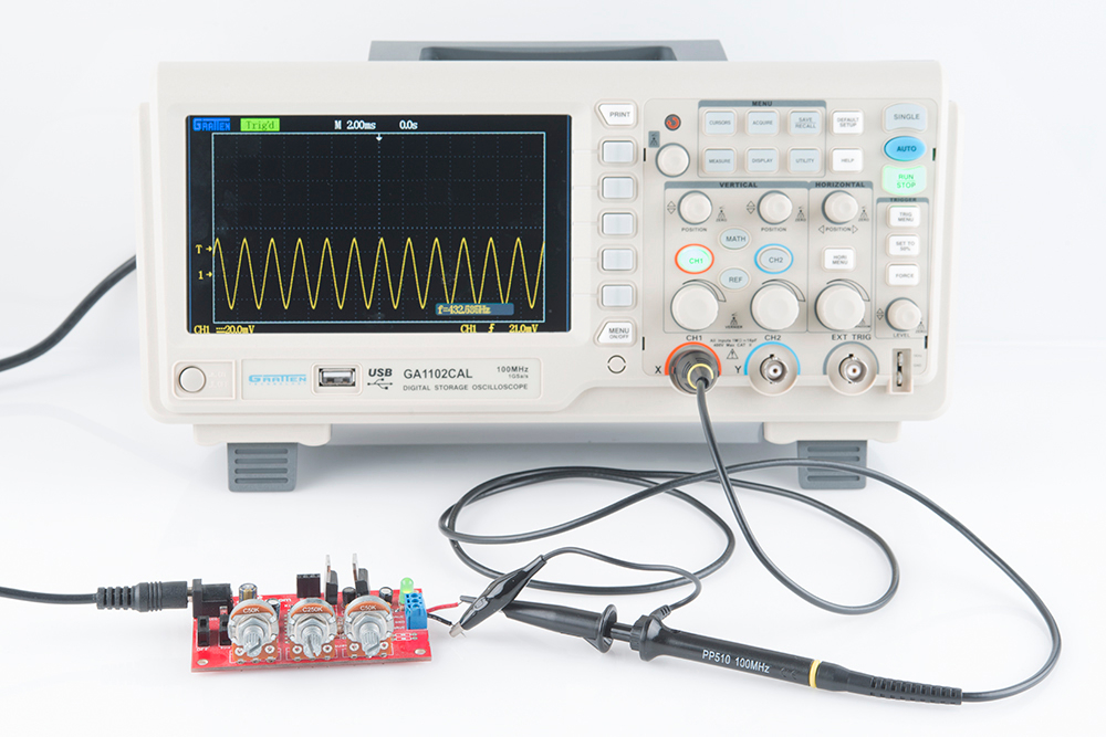
We’ll be using the Gratten GA1102CAL – a handy, mid-level, digital oscilloscope – as the basis for our scope discussion. Other o-scopes may look different, but they should all share a similar set of control and interface mechanisms.
Suggested Reading
Before continuing with this tutorial, you should be familiar with the concepts below. Check out the tutorial if you want to learn more!
- Voltage, Current, Resistance and Ohm’s Law
- How to Use a Multimeter
- Analog vs. Digital
- Alternating Current (AC) vs. Direct Current (DC)
Video
Basics of O-Scopes
The main purpose of an oscilloscope is to graph an electrical signal as it varies over time. Most scopes produce a two-dimensional graph with time on the x-axis and voltage on the y-axis.
An example of an oscilloscope display. A signal (the yellow sine wave in this case) is graphed on a horizontal time axis and a vertical voltage axis.
Controls surrounding the scope’s screen allow you to adjust the scale of the graph, both vertically and horizontally – allowing you to zoom in and out on a signal. There are also controls to set the trigger on the scope, which helps focus and stabilize the display.
What Can Scopes Measure
In addition to those fundamental features, many scopes have measurement tools, which help to quickly quantify frequency, amplitude, and other waveform characteristics. In general a scope can measure both time-based and voltage-based characteristics:
- Timing characteristics:
- Frequency and period – Frequency is defined as the number of times per second a waveform repeats. And the period is the reciprocal of that (number of seconds each repeating waveform takes). The maximum frequency a scope can measure varies, but it’s often in the 100’s of MHz (1E6 Hz) range.
- Duty cycle – The percentage of a period that a wave is either positive or negative (there are both positive and negative duty cycles). The duty cycle is a ratio that tells you how long a signal is “on” versus how long it’s “off” each period.
- Rise and fall time – Signals can’t instantaneously go from 0V to 5V, they have to smoothly rise. The duration of a wave going from a low point to a high point is called the rise time, and fall time measures the opposite. These characteristics are important when considering how fast a circuit can respond to signals.
- Voltage characteristics:
- Amplitude – Amplitude is a measure of the magnitude of a signal. There are a variety of amplitude measurements including peak-to-peak amplitude, which measures the absoluted difference between a high and low voltage point of a signal. Peak amplitude, on the other hand, only measures how high or low a signal is past 0V.
- Maximum and minimum voltages – The scope can tell you exactly how high and low the voltage of your signal gets.
- Mean and average voltages – Oscilloscopes can calculate the average or mean of your signal, and it can also tell you the average of your signal’s minimum and maximum voltage.
When to Use an O-Scope
The o-scope is useful in a variety of troubleshooting and research situations, including:
- Determining the frequency and amplitude of a signal, which can be critical in debugging a circuit’s input, output, or internal systems. From this, you can tell if a component in your circuit has malfunctioned.
- Identifying how much noise is in your circuit.
- Identifying the shape of a wave – sine, square, triangle, sawtooth, complex, etc.
- Quantifying phase differences between two different signals.
Oscilloscope Lexicon
Learning how to use an oscilloscope means being introduced to an entire lexicon of terms. On this page we’ll introduce some of the important o-scope buzzwords you should be familiar with before turning one on.
Key Oscilloscope Specifications
Some scopes are better than others. These characteristics help define how well you might expect a scope to perform:
- Bandwidth – Oscilloscopes are most commonly used to measure waveforms which have a defined frequency. No scope is perfect though: they all have limits as to how fast they can see a signal change. The bandwidth of a scope specifies the range of frequencies it can reliably measure.
- Digital vs. Analog – As with most everything electronic, o-scopes can either be analog or digital. Analog scopes use an electron beam to directly map the input voltage to a display. Digital scopes incorporate microcontrollers, which sample the input signal with an analog-to-digital converter and map that reading to the display. Generally analog scopes are older, have a lower bandwidth, and less features, but they may have a faster response (and look much cooler).
- Channel Amount – Many scopes can read more than one signal at a time, displaying them all on the screen simultaneously. Each signal read by a scope is fed into a separate channel. Two to four channel scopes are very common.
- Sampling Rate – This characteristic is unique to digital scopes, it defines how many times per second a signal is read. For scopes that have more than one channel, this value may decrease if multiple channels are in use.
- Rise Time – The specified rise time of a scope defines the fastest rising pulse it can measure. The rise time of a scope is very closely related to the bandwidth. It can be calculated as Rise Time = 0.35 / Bandwidth.
- Maximum Input Voltage – Every piece of electronics has its limits when it comes to high voltage. Scopes should all be rated with a maximum input voltage. If your signal exceeds that voltage, there’s a good chance the scope will be damaged.
- Resolution – The resolution of a scope represents how precisely it can measure the input voltage. This value can change as the vertical scale is adjusted.
- Vertical Sensitivity – This value represents the minimum and maximum values of your vertical, voltage scale. This value is listed in volts per div.
- Time Base – Time base usually indicates the range of sensitivities on the horizontal, time axis. This value is listed in seconds per div.
- Input Impedance – When signal frequencies get very high, even a small impedance (resistance, capacitance, or inductance) added to a circuit can affect the signal. Every oscilloscope will add a certain impedance to a circuit it’s reading, called the input impedance. Input impedances are generally represented as a large resistive impedance (>1 MΩ) in parallel (||) with small capacitance (in the pF range). The impact of input impedance is more apparent when measuring very high frequency signals, and the probe you use may have to help compensate for it.
Using the GA1102CAL as an example, here are specifications you might expect from a mid-range scope:
| Characteristic | Value |
|---|---|
| Bandwidth | 100 MHz |
| Sampling Rate | 1 GSa/s (1E9 samples per second) |
| Rise Time | <3.5ns |
| Channel Count | 2 |
| Maximum Input Voltage | 400V |
| Resolution | 8-bit |
| Vertical sensitivity | 2mV/div - 5V/div |
| Time base | 2ns/div - 50s/div |
| Input Impedance | 1 MΩ ±3% || 16pF ±3pF |
Understanding these characteristics, you should be able to pick out an oscilloscope that’ll best fit your needs. But you still have to know how to use it…onto the next page!
Anatomy of An O-Scope
While no scopes are created exactly equal, they should all share a few similarities that make them function similarly. On this page we’ll discuss a few of the more common systems of an oscilloscope: the display, horizontal, vertical, trigger, and inputs.
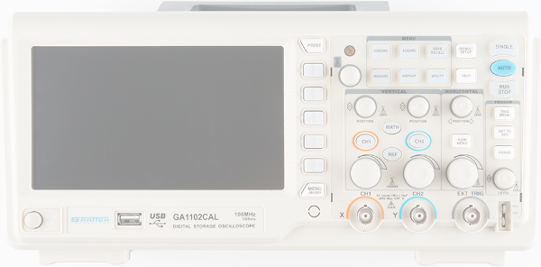
The Display
An oscilloscope isn’t any good unless it can display the information you’re trying to test, which makes the display one of the more important sections on the scope.
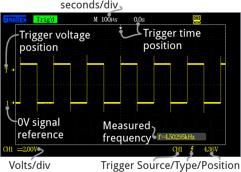
Every oscilloscope display should be criss-crossed with horizontal and vertical lines called divisions. The scale of those divisions are modified with the horizontal and vertical systems. The vertical system is measured in “volts per division” and the horizontal is “seconds per division”. Generally, scopes will feature around 8-10 vertical (voltage) divisions, and 10-14 horizontal (seconds) divisions.
Older scopes (especially those of the analog variety) usually feature a simple, monochrome display, though the intensity of the wave may vary. More modern scopes feature multicolor LCD screens, which are a great help in showing more than one waveform at a time.
Many scope displays are situated next to a set of about five buttons – either to the side or below the display. These buttons can be used to navigate menus and control settings of the scope.
Vertical System
The vertical section of the scope controls the voltage scale on the display. There are traditionally two knobs in this section, which allow you to individually control the vertical position and volts/div.
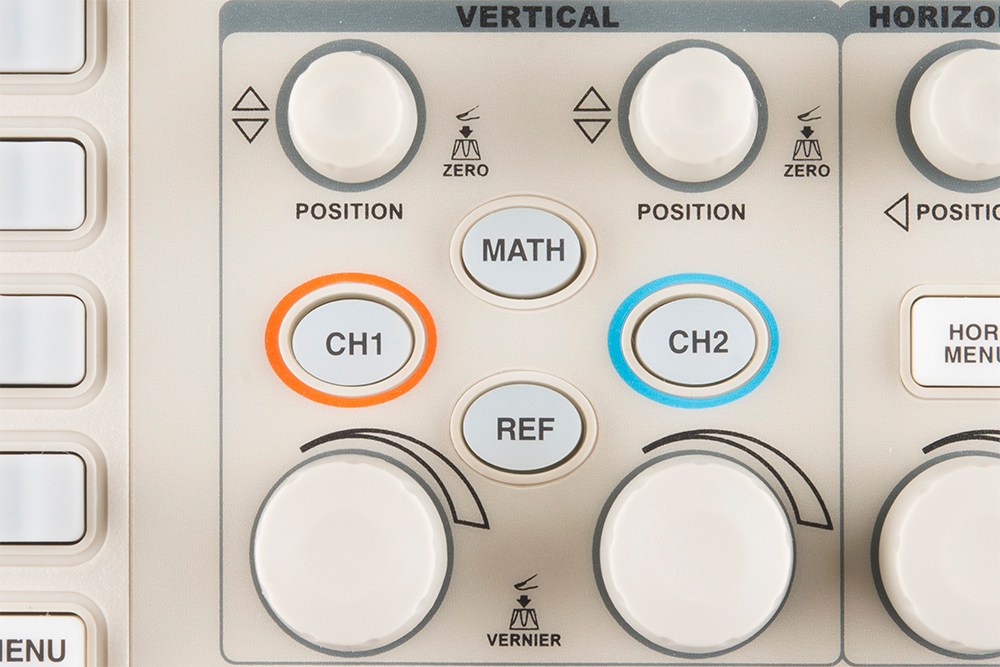
The more critical volts per division knob allows you to set the vertical scale on the screen. Rotating the knob clockwise will decrease the scale, and counter-clockwise will increase. A smaller scale – fewer volts per division on the screen – means you’re more “zoomed in” to the waveform.
The display on the GA1102, for example, has 8 vertical divisions, and the volts/div knob can select a scale between 2mV/div and 5V/div. So, zoomed all the way in to 2mV/div, the display can show waveform that is 16mV from top to bottom. Fully “zoomed out”, the scope can show a waveform ranging over 40V. (The probe, as we’ll discuss below, can further increase this range.)
The position knob controls the vertical offset of the waveform on the screen. Rotate the knob clockwise, and the wave will move down, counter-clockwise will move it up the display. You can use the position knob to offset part of a waveform off the screen.
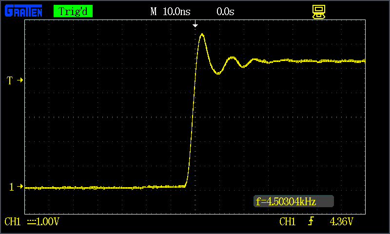
Using both the position and volts/div knobs in conjunction, you can zoom in on just a tiny part of the waveform that you care about the most. If you had a 5V square wave, but only cared about how much it was ringing on the edges, you could zoom in on the rising edge using both knobs.
Horizontal System
The horizontal section of the scope controls the time scale on the screen. Like the vertical system, the horizontal control gives you two knobs: position and seconds/div.
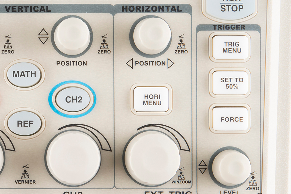
The seconds per division (s/div) knob rotates to increase or decrease the horizontal scale. If you rotate the s/div knob clockwise, the number of seconds each division represents will decrease – you’ll be “zooming in” on the time scale. Rotate counter-clockwise to increase the time scale, and show a longer amount of time on the screen.
Using the GA1102 as an example again, the display has 14 horizontal divisions, and can show anywhere between 2nS and 50s per division. So zoomed all the way in on the horizontal scale, the scope can show 28nS of a waveform, and zoomed way out it can show a signal as it changes over 700 seconds.
The position knob can move your waveform to the right or left of the display, adjusting the horizontal offset.
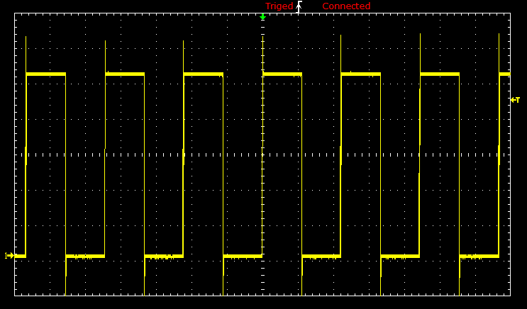
Using the horizontal system, you can adjust how many periods of a waveform you want to see. You can zoom out, and show multiple peaks and troughs of a signal:
Or you can zoom way in, and use the position knob to show just a tiny part of a wave:
Trigger System
The trigger section is devoted to stabilizing and focusing the oscilloscope. The trigger tells the scope what parts of the signal to “trigger” on and start measuring. If your waveform is periodic, the trigger can be manipulated to keep the display static and unflinching. A poorly triggered wave will produce seizure-inducing sweeping waves like this:
The trigger section of a scope is usually comprised of a level knob and a set of buttons to select the source and type of the trigger. The level knob can be twisted to set a trigger to a specific voltage point.
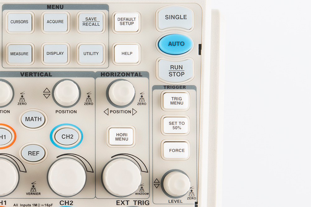
A series of buttons and screen menus make up the rest of the trigger system. Their main purpose is to select the trigger source and mode. There are a variety of trigger types, which manipulate how the trigger is activated:
- An edge trigger is the most basic form of the trigger. It will key the oscilloscope to start measuring when the signal voltage passes a certain level. An edge trigger can be set to catch on a rising or falling edge (or both).
- A pulse trigger tells the scope to key in on a specified “pulse” of voltage. You can specify the duration and direction of the pulse. For example, it can be a tiny blip of 0V -> 5V -> 0V, or it can be a seconds-long dip from 5V to 0V, back to 5V.
- A slope trigger can be set to trigger the scope on a positive or negative slope over a specified amount of time.
- More complicated triggers exist to focus on standardized waveforms that carry video data, like NTSC or PAL. These waves use a unique synchronizing pattern at the beginning of every frame.
You can also usually select a triggering mode, which, in effect, tells the scope how strongly you feel about your trigger. In automatic trigger mode, the scope can attempt to draw your waveform even if it doesn’t trigger. Normal mode will only draw your wave if it sees the specified trigger. And single mode looks for your specified trigger, when it sees it it will draw your wave then stop.
The Probes
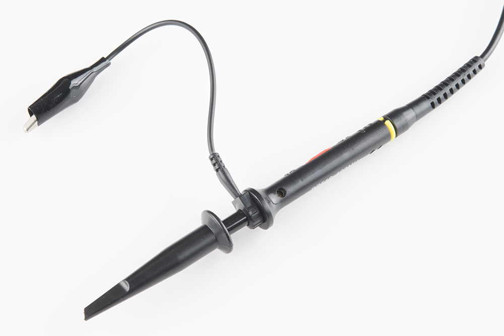
An oscilloscope is only good if you can actually connect it to a signal, and for that you need probes. Probes are single-input devices that route a signal from your circuit to the scope. They have a sharp tip which probes into a point on your circuit. The tip can also be equipped with hooks, tweezers or clips to make latching onto a circuit easier. Every probe also includes a ground clip, which should be secured safely to a common ground point on the circuit under test.
While probes may seem like simple devices that just latch onto your circuit and carry a signal to the scope, there’s actually a lot that goes into probe design and selection.
Optimally, what a probe needs to be is invisible – it shouldn’t have any effect on your signal under test. Unfortunately, long wires all have intrinsic inductance, capacitance, and resistance, so, no matter what, they’ll affect scope readings (especially at high frequencies).
There are a variety of probe types out there, the most common of which is the passive probe, included with most scopes. Most of the “stock” passive probes are attenuated. Attenuating probes have a large resistance intentionally built-in and shunted by a small capacitor, which helps to minimize the effect that a long cable might have on loading your circuit. In series with the input impedance of a scope, this attenuated probe will create a voltage divider between your signal and the scope input.
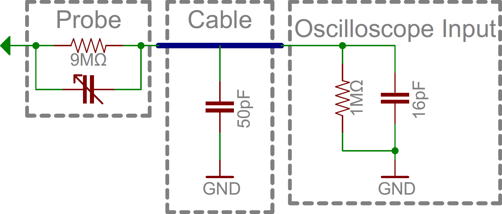
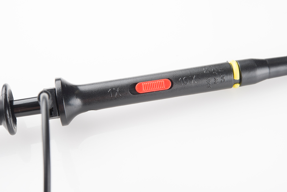
Most probes have a 9MΩ resistor for attenuating, which, when combined with a standard 1MΩ input impedance on a scope, creates a 1/10 voltage divider. These probes are commonly called 10X attenuated probes. Many probes include a switch to select between 10X and 1X (no attenuation).
Attenuated probes are great for improving accuracy at high frequencies, but they will also reduce the amplitude of your signal. If you’re trying to measure a very low-voltage signal, you may have to go with a 1X probe. You may also need to select a setting on your scope to tell it you’re using an attenuated probe, although many scopes can automatically detect this.
Beyond the passive attenuated probe, there are a variety of other probes out there. Active probes are powered probes (they require a separate power source), which can amplify your signal or even pre-process it before it get to your scope. While most probes are designed to measure voltage, there are probes designed to measure AC or DC current. Current probes are unique because they often clamp around a wire, never actually making contact with the circuit.
Using an Oscilloscope
The infinite variety of signals out there means you’ll never operate an oscilloscope the same way twice. But there are some steps you can count on performing just about every time you test a circuit. On this page we’ll show an example signal, and the steps required to measure it.
Probe Selection and Setup
First off, you’ll need to select a probe. For most signals, the simple passive probe included with your scope will work perfectly fine.
Next, before connecting it to your scope, set the attenuation on your probe. 10X – the most common attenuation factor – is usually the most well-rounded choice. If you’re trying to measure a very low-voltage signal though, you may need to use 1X.
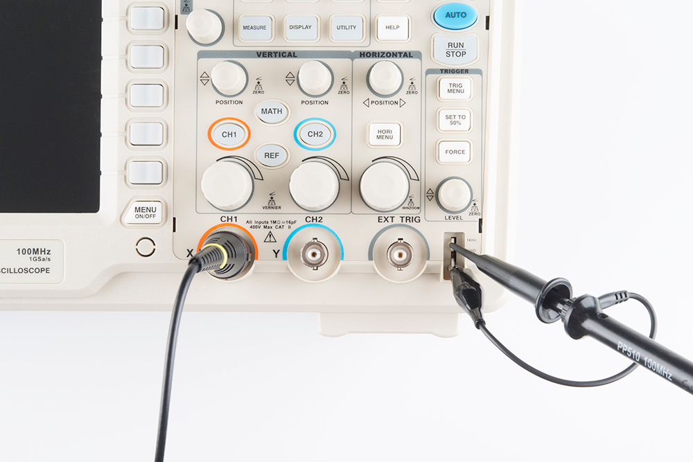
Connect the Probe and Turn the Scope On
Connect your probe to the first channel on your scope, and turn it on. Have some patience here, some scopes take as long to boot up as an old PC.
When the scope boots up you should see the divisions, scale, and a noisy, flat line of a waveform.
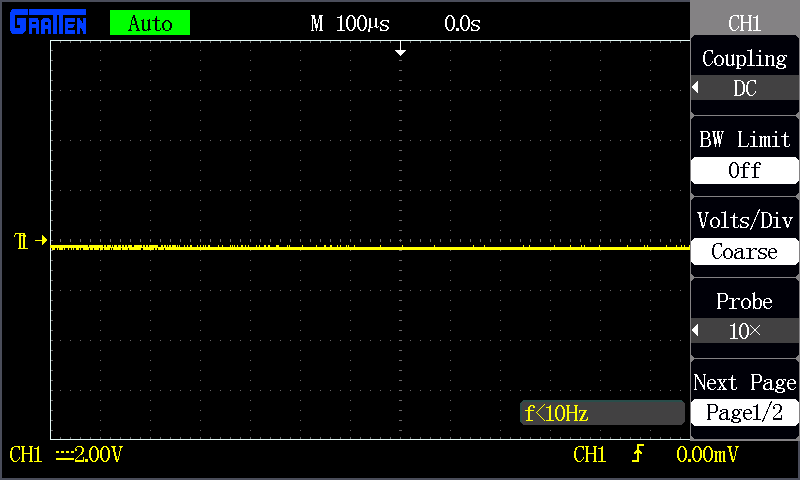
The screen should also show previously set values for time and volts per div. Ignoring those scales for now, make these adjustments to put your scope into a standard setup:
- Turn channel 1 on and channel 2 off.
- Set channel 1 to DC coupling.
- Set the trigger source to channel 1 – no external source or alternate channel triggering.
- Set the trigger type to rising edge, and the trigger mode to auto (as opposed to single).
- Make sure the scope probe attenuation on your scope matches the setting on your probe (e.g. 1X, 10X).
For help making these adjustments, consult your scope’s user’s manual (as an example, here’s the GA1102CAL manual).
Testing the Probe
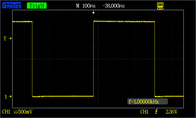
Let’s connect that channel up to a meaningful signal. Most scopes will have a built-in frequency generator that emits a reliable, set-frequency wave – on the GA1102CAL there is a 1kHz square wave output at the bottom-right of the front panel. The frequency generator output has two separate conductors – one for the signal and one for ground. Connect your probe’s ground clip to the ground, and the probe tip to the signal output.
As soon as you connect both parts of the probe, you should see a signal begin to dance around your screen. Try fiddling with the horizontal and vertical system knobs to maneuver the waveform around the screen. Rotating the scale knobs clockwise will “zoom into” your waveform, and counter-clockwise zooms out. You can also use the position knob to further locate your waveform.
If your wave is still unstable, try rotating the trigger position knob. Make sure the trigger isn’t higher than the tallest peak of your waveform. By default, the trigger type should be set to edge, which is usually a good choice for square waves like this.
Try fiddling with those knobs enough to display a single period of your wave on the screen.
Or try zooming way out on the time scale to show dozens of squares.
Compensating an Attenuated Probe
If your probe is set to 10X, and you don’t have a perfectly square waveform as shown above, you may need to compensate your probe. Most probes have a recessed screw head, which you can rotate to adjust the shunt capacitance of the probe.

Try using a small screwdriver to rotate this trimmer, and look at what happens to the waveform.
Adjust the trimming cap on the probe handle until you have a straight-edged square wave. Compensation is only necessary if your probe is attenuated (e.g. 10X), in which case it’s critical (especially if you don’t know who used your scope last!).
Probing, Triggering, and Scaling Tips
Once you’ve compensated your probe, it’s time to measure a real signal! Go find a signal source (frequency generator?, Terror-Min?) and come back.
The first key to probing a signal is finding a solid, reliable grounding point. Clasp your ground clip to a known ground, sometimes you may have to use a small wire to intermediate between the ground clip and your circuit’s ground point. Then connect your probe tip to the signal under test. Probe tips exist in a variety of form factors – the spring-loaded clip, fine point, hooks, etc. – try to find one that doesn’t require you to hold it in place all the time.
Once your signal is on the screen, you may want to begin by adjusting the horizontal and vertical scales into at least the “ballpark” of your signal. If you’re probing a 5V 1kHz square wave, you’ll probably want the volts/div somewhere around 0.5-1V, and set the seconds/div to around 100µs (14 divisions would show about one and a half periods).
If part of your wave is rising or falling of the screen, you can adjust the vertical position to move it up or down. If your signal is purely DC, you may want to adjust the 0V level near the bottom of your display.
Once you have the scales ballparked, your waveform may need some triggering. Edge triggering – where the scope tries to begin its scan when it sees voltage rise (or fall) past a set point – is the easiest type to use. Using an edge trigger, try to set the trigger level to a point on your waveform that only sees a rising edge once per period.
Now just scale, position, trigger and repeat until you’re looking at exactly what you need.
Measure Twice, Cut Once
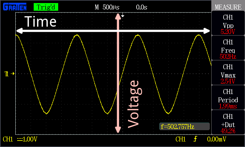
With a signal scoped, triggered, and scaled, it comes time to measure transients, periods, and other waveform properties. Some scopes have more measurement tools than others, but they’ll all at least have divisions, from which you should be able to at least estimate the amplitude and frequency.
Many scopes support a variety of automatic measurement tools, they may even constantly display the most relevant information, like frequency. To get the most out of your scope, you’ll want to explore all of the measure functions it supports. Most scopes will calculate frequency, amplitude, duty cycle, mean voltage, and a variety of other wave characteristics for you automatically.
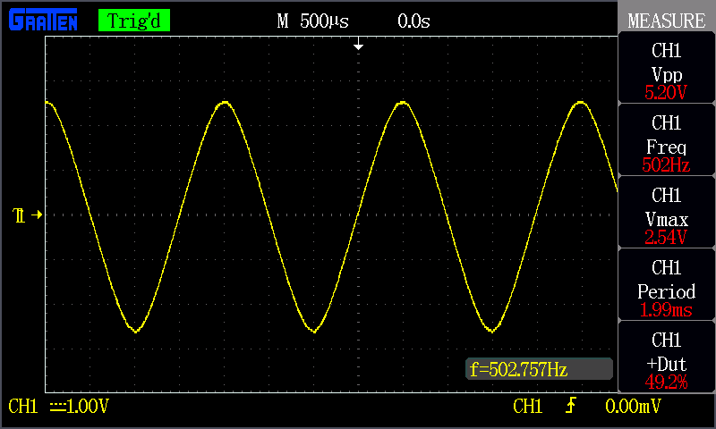
Using the scope’s measure tools to find VPP, VMax, frequency, period, and duty cycle.
A third measuring tool many scopes provide is cursors. Cursors are on-screen, movable markers which can be placed on either the time or voltage axis. Cursors usually come in pairs, so you can measure the difference between one and the other.

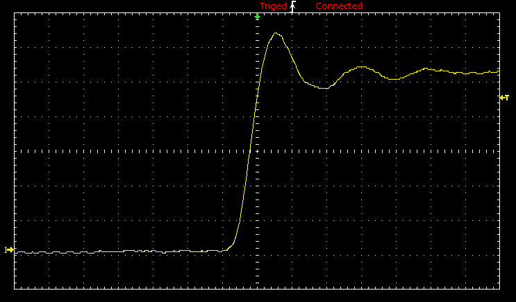
Measuring the ringing of a square wave with cursors.
Once you’ve measured the quantity you were looking for, you can begin to make adjustments to your circuit and measure some more! Some scopes also support saving, printing, or storing a waveform, so you can recall it and remember those good ol' times when you scoped that signal.
To find out more about what your scope can do, consult its user’s manual!
Purchasing an Oscilloscope
Now that you’ve learned all about this handy tool’s features and benefits, it’s time to put an oscilloscope on the workbench.